 A function is vector-valued (instead of scalar-valued)
if the values of its outputs are vectors (instead of scalars).
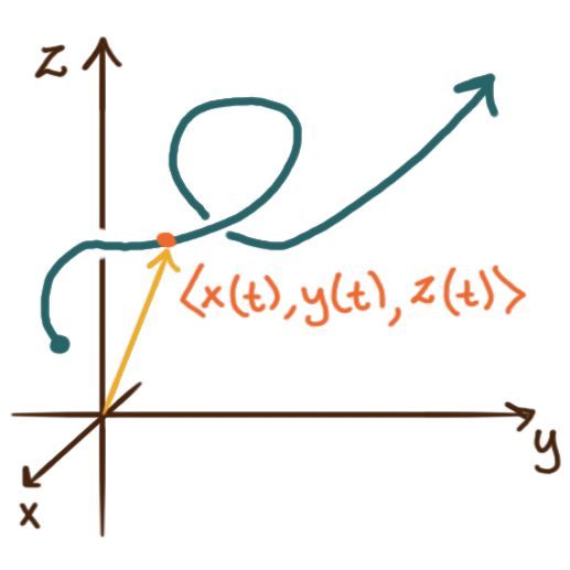
A vector-valued function \(\bm{r}\colon \mathbf{R} \to \mathbf{R}^3\)
can be visualized as a parametrically-defined curve in three-dimensional space;
the domain \(\mathbf{R}\) is literally a line being embedded in \(\mathbf{R}^3.\)
For a curve \(C\) with parameterization
\(\bm{r}(t) = \bigl\langle x(t), y(t), z(t)\bigr\rangle\)
we refer to \(t\) as the parameter
and to \(x(t)\) and \(y(t)\) and \(z(t)\)
as the component functions or coordinate functions.
A single curve has infinitely many parameterizations.
For any function \(f\) and any parameterization \(\bm{r}\) of a curve \(C,\)
the composite \(\bm{r} \circ f\) will also be a parameterization of \(C.\)
The starting point (where \(t=0\)) and “speed” of a parameterization
can be altered per choice of a function \(f.\)
A function is vector-valued (instead of scalar-valued)
if the values of its outputs are vectors (instead of scalars).
A vector-valued function \(\bm{r}\colon \mathbf{R} \to \mathbf{R}^3\)
can be visualized as a parametrically-defined curve in three-dimensional space;
the domain \(\mathbf{R}\) is literally a line being embedded in \(\mathbf{R}^3.\)
For a curve \(C\) with parameterization
\(\bm{r}(t) = \bigl\langle x(t), y(t), z(t)\bigr\rangle\)
we refer to \(t\) as the parameter
and to \(x(t)\) and \(y(t)\) and \(z(t)\)
as the component functions or coordinate functions.
A single curve has infinitely many parameterizations.
For any function \(f\) and any parameterization \(\bm{r}\) of a curve \(C,\)
the composite \(\bm{r} \circ f\) will also be a parameterization of \(C.\)
The starting point (where \(t=0\)) and “speed” of a parameterization
can be altered per choice of a function \(f.\)
 A curve \(C\) is closed if for some parameterization
the entire curve is traced out for some bounded interval of the parameter \(t.\)
I.e. it “loops back on itself” and continually retraces itself.
A curve \(C\) is rectifiable if its arclength
can be approximated to arbitrary precision
as the sum of the lengths of finitely many line segments
with endpoint on the curve; fractal curves are not rectifiable.
A vector-valued function \(\bm{r}\colon \mathbf{R}^2 \to \mathbf{R}^3\)
can be visualized as a parametrically-defined surface in three-dimensional space;
the domain \(\mathbf{R}^2\) is literally a plane being embedded in \(\mathbf{R}^3.\)
For a surface \(S\) with parameterization \(\bm{r}(s,t)\)
we refer to \(s\) and \(t\) as the parameters.
Note that many writers conventionally use \(u\) and \(v\) as the names of the parameters for a surface.
A surface \(S\) is closed if for some parameterization
if the entire surface is traced out for some bounded interval of the parameters \(s\) and \(t.\)
A curve \(C\) is closed if for some parameterization
the entire curve is traced out for some bounded interval of the parameter \(t.\)
I.e. it “loops back on itself” and continually retraces itself.
A curve \(C\) is rectifiable if its arclength
can be approximated to arbitrary precision
as the sum of the lengths of finitely many line segments
with endpoint on the curve; fractal curves are not rectifiable.
A vector-valued function \(\bm{r}\colon \mathbf{R}^2 \to \mathbf{R}^3\)
can be visualized as a parametrically-defined surface in three-dimensional space;
the domain \(\mathbf{R}^2\) is literally a plane being embedded in \(\mathbf{R}^3.\)
For a surface \(S\) with parameterization \(\bm{r}(s,t)\)
we refer to \(s\) and \(t\) as the parameters.
Note that many writers conventionally use \(u\) and \(v\) as the names of the parameters for a surface.
A surface \(S\) is closed if for some parameterization
if the entire surface is traced out for some bounded interval of the parameters \(s\) and \(t.\)