 A multivariable function, scalar-valued function
is a function that takes a vector as input and returns a scalar (number) as output.
In particular, for a two-variable function
\(f \colon \mathbf{R}^2 \to \mathbf{R},\)
the input is a vector \(\langle x,y \rangle\) in \(\mathbf{R}^2\)
and the output is a scalar in \(\mathbf{R}.\)
The common convention is to denote this output as \(f(x,y),\)
but strictly speaking it should be \(f\bigl(\langle x,y \rangle\bigr).\)
Sometimes multivariable, scalar-valued functions
are referred to as scalar fields.
We can visualize such a two-variable function
A multivariable function, scalar-valued function
is a function that takes a vector as input and returns a scalar (number) as output.
In particular, for a two-variable function
\(f \colon \mathbf{R}^2 \to \mathbf{R},\)
the input is a vector \(\langle x,y \rangle\) in \(\mathbf{R}^2\)
and the output is a scalar in \(\mathbf{R}.\)
The common convention is to denote this output as \(f(x,y),\)
but strictly speaking it should be \(f\bigl(\langle x,y \rangle\bigr).\)
Sometimes multivariable, scalar-valued functions
are referred to as scalar fields.
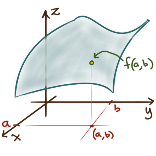
We can visualize such a two-variable function
 via its graph \(z = f(x,y)\) in three-dimensional space,
where the output is plotted as the \(z\)-coordinate
“above” or “below” the \(xy\)-plane.
Generically the graph of such a function is a surface.
For any specific output value \(z_0,\)
the horizontal cross-section of the graph \(z_0 = f(x,y)\)
is called its level curve at \(z_0,\)
or more generally its level set.
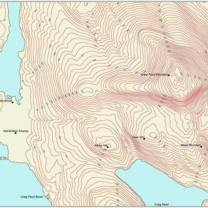
A contour plot of a function
is a plot of a collection of its level curves
which provides a top-down “topographic” view
of the function’s graph.
For a three-variable function
\(f \colon \mathbf{R}^3 \to \mathbf{R},\)
its graph \(w = f(x,y,z)\) would be four-dimensional,
and difficult to visualize;
we can only reasonably visualize
a three-variable function via a contour plot,
consisting of level surfaces \(w_0 = f(x,y,z).\)
via its graph \(z = f(x,y)\) in three-dimensional space,
where the output is plotted as the \(z\)-coordinate
“above” or “below” the \(xy\)-plane.
Generically the graph of such a function is a surface.
For any specific output value \(z_0,\)
the horizontal cross-section of the graph \(z_0 = f(x,y)\)
is called its level curve at \(z_0,\)
or more generally its level set.
A contour plot of a function
is a plot of a collection of its level curves
which provides a top-down “topographic” view
of the function’s graph.
For a three-variable function
\(f \colon \mathbf{R}^3 \to \mathbf{R},\)
its graph \(w = f(x,y,z)\) would be four-dimensional,
and difficult to visualize;
we can only reasonably visualize
a three-variable function via a contour plot,
consisting of level surfaces \(w_0 = f(x,y,z).\)