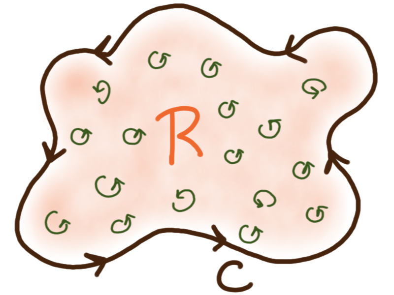
A closed simple curve in the plane is positively oriented if it is being traversed counter-clockwise (right-handedly). For a line integral over \(C\) that respects the positive orientation of \(C\) we use the notation \(\oint_C.\) For a region \(R\) let \(\partial R\) denote the boundary of \(R.\)
 Green’s Theorem (circulation) —
for a simply-connected planar region \(R\) whose boundary is
a simple, piecewise-smooth curve \(C = \partial R,\)
and a two-dimensional vector field \(\bm{F} = L\mathbf{i} + M\mathbf{j}\)
whose components \(L\) and \(M\) have continuous partial derivatives
on some open neighborhood containing \(R,\)
\[
\iint_R \bigg(\frac{\partial M}{\partial x}-\frac{\partial L}{\partial y}\bigg) \,\mathrm{d}A
= \oint_{C} L\,\mathrm{d}x + M\,\mathrm{d}y
= \oint_{C} \bm{F}\cdot\mathbf{T}\,\mathrm{d}s
= \oint_{C} \bm{F}\cdot\mathrm{d}\bm{r}
\,.
\]
I.e. the total “vorticity” within the interior of a region
can be computed as a line integral along its boundary.
In a sense, the integrand \({\tfrac{\partial M}{\partial x}\!-\!\tfrac{\partial L}{\partial y}}\)
measures how much the vector field is “circulating” at a point,
how much it fails to be conservative.
Green’s Theorem (circulation) —
for a simply-connected planar region \(R\) whose boundary is
a simple, piecewise-smooth curve \(C = \partial R,\)
and a two-dimensional vector field \(\bm{F} = L\mathbf{i} + M\mathbf{j}\)
whose components \(L\) and \(M\) have continuous partial derivatives
on some open neighborhood containing \(R,\)
\[
\iint_R \bigg(\frac{\partial M}{\partial x}-\frac{\partial L}{\partial y}\bigg) \,\mathrm{d}A
= \oint_{C} L\,\mathrm{d}x + M\,\mathrm{d}y
= \oint_{C} \bm{F}\cdot\mathbf{T}\,\mathrm{d}s
= \oint_{C} \bm{F}\cdot\mathrm{d}\bm{r}
\,.
\]
I.e. the total “vorticity” within the interior of a region
can be computed as a line integral along its boundary.
In a sense, the integrand \({\tfrac{\partial M}{\partial x}\!-\!\tfrac{\partial L}{\partial y}}\)
measures how much the vector field is “circulating” at a point,
how much it fails to be conservative.
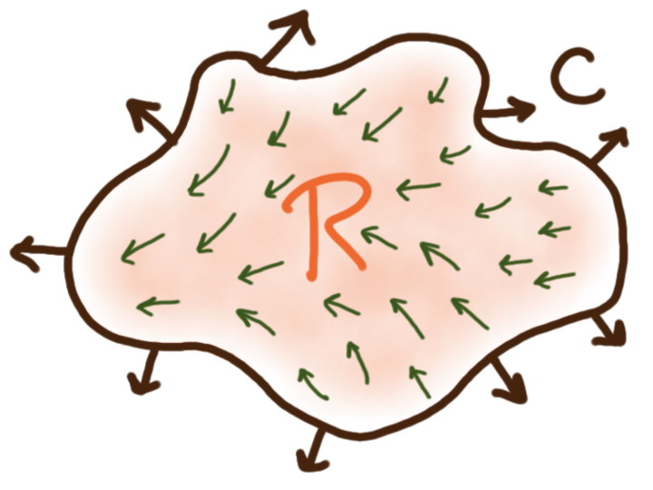 Green’s Theorem (flux) —
for the same region \(R\) and boundary \(C = \partial R\)
and vector field \(\bm{F} = L\mathbf{i} + M\mathbf{j},\)
\[
\iint_R \bigg(\frac{\partial L}{\partial x}+\frac{\partial M}{\partial y}\bigg) \,\mathrm{d}A
%= \oint_{C} L\,\mathrm{d}x + M\,\mathrm{d}y
= \oint_{C} \bm{F}\cdot\mathbf{N}\,\mathrm{d}s
%= \oint_{C} \bm{F}\times\mathrm{d}\bm{r}
\,.
\]
I.e. the total “flow density” within the interior of a region
can be computed as a line integral of that flow across its boundary,
the flux across the boundary.
Green’s Theorem (flux) —
for the same region \(R\) and boundary \(C = \partial R\)
and vector field \(\bm{F} = L\mathbf{i} + M\mathbf{j},\)
\[
\iint_R \bigg(\frac{\partial L}{\partial x}+\frac{\partial M}{\partial y}\bigg) \,\mathrm{d}A
%= \oint_{C} L\,\mathrm{d}x + M\,\mathrm{d}y
= \oint_{C} \bm{F}\cdot\mathbf{N}\,\mathrm{d}s
%= \oint_{C} \bm{F}\times\mathrm{d}\bm{r}
\,.
\]
I.e. the total “flow density” within the interior of a region
can be computed as a line integral of that flow across its boundary,
the flux across the boundary.
We can extend Green’s theorem to regions that aren’t simply-connected by dissecting them into finitely many simply-connected regions.