A Riemann sum is a sum of the signed areas of a collection of rectangles, each of the same uniform width and each with a height determined by the graph of a function \(f,\) that approximates the area of the region bound by the graph and the \(x\)-axis between \({x=a}\) and \({x=b.}\) The units of the Riemann sum will be the product of the units of the variables \(x\) and \(y.\) E.g. if \(x\) is measured in feet-per-second and \(y\) is measured in seconds, then the Riemann sum (area) will have units feet.
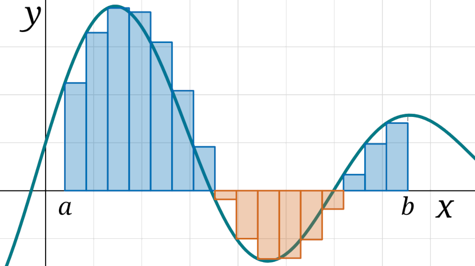 For a Riemann sum with \(n\) rectangles, the interval \([a,b]\) is partitioned
into \(n\) subintervals, each of width \(h = \frac{b-a}{n}.\)
There are various conventions for how each rectangle’s height is chosen:
e.g. choosing the rectangle’s height to be the function’s value
at the left-endpoint of the rectangle’s base
results in what’s called a left-endpoint Riemann sum.
For large values of \(n\) (many rectangles)
this sum is unwieldy to write,
so we invent a new notation, sigma summation notation.
The notation
\[ \sum_{i=1}^{n} \bigl(f(a+ih) \times h\bigr) \]
is read as “the sum of the areas \(\bigl(f(a+ih) \times h\bigr)\)
counting from \(i=1\) up to \(i=n\).”
Some computational facts about sigma notation:
\[
\sum_{i=1}^{n} k a_i \!=\! k \sum_{i=1}^{n} a_i
\qquad\quad
\sum_{i=1}^{n} a_i \pm b_i \!=\! \sum_{i=1}^{n} a_i \!\pm\! \sum_{i=1}^{n} b_i
\qquad\quad
\sum_{i=1}^{n} i \!=\! \frac{n(n+1)}{2}
\qquad\quad
\sum_{i=1}^{n} i^2 \!=\! \frac{n(n+1)(2n+1)}{6}
\qquad\quad
\sum_{i=1}^{n} i^3 \!=\! \biggl(\frac{n(n+1)}{2}\biggr)^2
\]
For a Riemann sum with \(n\) rectangles, the interval \([a,b]\) is partitioned
into \(n\) subintervals, each of width \(h = \frac{b-a}{n}.\)
There are various conventions for how each rectangle’s height is chosen:
e.g. choosing the rectangle’s height to be the function’s value
at the left-endpoint of the rectangle’s base
results in what’s called a left-endpoint Riemann sum.
For large values of \(n\) (many rectangles)
this sum is unwieldy to write,
so we invent a new notation, sigma summation notation.
The notation
\[ \sum_{i=1}^{n} \bigl(f(a+ih) \times h\bigr) \]
is read as “the sum of the areas \(\bigl(f(a+ih) \times h\bigr)\)
counting from \(i=1\) up to \(i=n\).”
Some computational facts about sigma notation:
\[
\sum_{i=1}^{n} k a_i \!=\! k \sum_{i=1}^{n} a_i
\qquad\quad
\sum_{i=1}^{n} a_i \pm b_i \!=\! \sum_{i=1}^{n} a_i \!\pm\! \sum_{i=1}^{n} b_i
\qquad\quad
\sum_{i=1}^{n} i \!=\! \frac{n(n+1)}{2}
\qquad\quad
\sum_{i=1}^{n} i^2 \!=\! \frac{n(n+1)(2n+1)}{6}
\qquad\quad
\sum_{i=1}^{n} i^3 \!=\! \biggl(\frac{n(n+1)}{2}\biggr)^2
\]