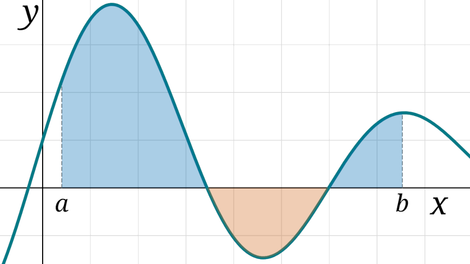
For a function \(f\) defined on \((a,b),\) the definite integral of \(f\) from \(a\) to \(b,\) denoted \( \int_a^b f(x) \,\mathrm{d}x\,, \) represents the signed area of the region bound by the graph of \(f\) and the \(x\)-axis between \(x=a\) and \(x=b.\) We refer to \(f\) as the integrand and to \(a\) and \(b\) as the lower bound and upper bound of the integral respectively. The definite integral counts the amount of area that \(f\) accumulates as \(x\) sweeps from \(a\) to \(b.\) The area is signed in the sense that any portion of the region underneath the \(x\)-axis counts negatively towards the accumulated area.
 Formally the definite integral is defined as the limit of a Riemann sum
as the number of rectangles approaches infinity,
and we say \(f\) is integrable only if this limit exists:
\[ \int\limits_a^b f(x)\,\mathrm{d}x \;\;=\;\; \lim\limits_{n \to \infty} \sum_{i=1}^{n} \bigl(f(a+ih) \times h\bigr) \quad \text{for}\;\; h = \frac{b-a}{n}\]
A few computational facts about definite integrals
can be inferred from the geometry of the area they represent
and their definition in terms of a Riemann sum:
\[
\int\limits_a^b f(x) \,\mathrm{d}x = -\int\limits_b^a f(x) \,\mathrm{d}x
\qquad
\int\limits_a^b k f(x) \,\mathrm{d}x = k\int\limits_a^b f(x) \,\mathrm{d}x
\qquad
\int\limits_a^a k f(x) \,\mathrm{d}x = 0
\]
\[
\int\limits_a^b \bigl(f(x) \pm g(x)\bigr) \,\mathrm{d}x = \int\limits_a^b f(x) \,\mathrm{d}x \pm \int\limits_a^b f(x) \,\mathrm{d}x
\qquad
\int\limits_a^b f(x) \,\mathrm{d}x + \int\limits_b^c f(x) \,\mathrm{d}x = \int\limits_a^c f(x) \,\mathrm{d}x
\qquad
% \int\limits_a^b x \,\mathrm{d}x = \frac{b^2-a^2}{2}
% \qquad
% \int\limits_a^b x^2 \,\mathrm{d}x = \frac{b^3-a^3}{3}
% \qquad
% \int\limits_a^b x^3 \,\mathrm{d}x = \frac{b^4-a^4}{4}
\]
Formally the definite integral is defined as the limit of a Riemann sum
as the number of rectangles approaches infinity,
and we say \(f\) is integrable only if this limit exists:
\[ \int\limits_a^b f(x)\,\mathrm{d}x \;\;=\;\; \lim\limits_{n \to \infty} \sum_{i=1}^{n} \bigl(f(a+ih) \times h\bigr) \quad \text{for}\;\; h = \frac{b-a}{n}\]
A few computational facts about definite integrals
can be inferred from the geometry of the area they represent
and their definition in terms of a Riemann sum:
\[
\int\limits_a^b f(x) \,\mathrm{d}x = -\int\limits_b^a f(x) \,\mathrm{d}x
\qquad
\int\limits_a^b k f(x) \,\mathrm{d}x = k\int\limits_a^b f(x) \,\mathrm{d}x
\qquad
\int\limits_a^a k f(x) \,\mathrm{d}x = 0
\]
\[
\int\limits_a^b \bigl(f(x) \pm g(x)\bigr) \,\mathrm{d}x = \int\limits_a^b f(x) \,\mathrm{d}x \pm \int\limits_a^b f(x) \,\mathrm{d}x
\qquad
\int\limits_a^b f(x) \,\mathrm{d}x + \int\limits_b^c f(x) \,\mathrm{d}x = \int\limits_a^c f(x) \,\mathrm{d}x
\qquad
% \int\limits_a^b x \,\mathrm{d}x = \frac{b^2-a^2}{2}
% \qquad
% \int\limits_a^b x^2 \,\mathrm{d}x = \frac{b^3-a^3}{3}
% \qquad
% \int\limits_a^b x^3 \,\mathrm{d}x = \frac{b^4-a^4}{4}
\]