A discrete random variable assumes one of only finitely many possible outcomes, whereas a continuous random variable assumes one of infinitely many possible outcomes. E.g. rolling a standard die versus measuring the height of a randomly selected person.
For a continuous random variable \(X,\) let \(\operatorname{P}(a \leq X \leq b)\) or \(\operatorname{P}\bigl([a, b]\bigr)\) denote the probability that the value of \(X\) is between \(a\) and \(b.\)
For a continuous random variable \(X\) with set of possible outcomes \(D,\) a probability density function (PDF) is a function \(f\) with domain \(D\) such that \(f(x) \geq 0\) on \(D,\) and \(\int_{D} f(x) \,\mathrm{d}x = 1\,,\) and \(\operatorname{P}(a \leq X \leq b) = \int_a^b f(x)\,\mathrm{d}x\,.\) This last condition is the namesake of a probability density function: the value of the integral \(\int_a^b f(x)\,\mathrm{d}x\) is the probability that \(X\) is between \(a\) and \(b.\) Common examples of PDFs include:
 The expected value of \(X\), denoted \(\operatorname{E}\bigl(X\bigr)\)
and often simply referred to as the mean and denoted \(\mu,\)
is computed as \(\operatorname{E}\bigl(X\bigr) = \int_{D} x f(x) \,\mathrm{d}x\,.\)
The variance of \(X,\) denoted \(\operatorname{Var}(X)\) or \(\sigma^2,\)
is computed as \(\operatorname{Var}\bigl(X\bigr) = \int_{D} (x\!-\!\mu)^2 f(x) \,\mathrm{d}x\,.\)
The standard deviation of \(X\) is the positive square root of the variance,
and is denoted as \(\sigma.\)
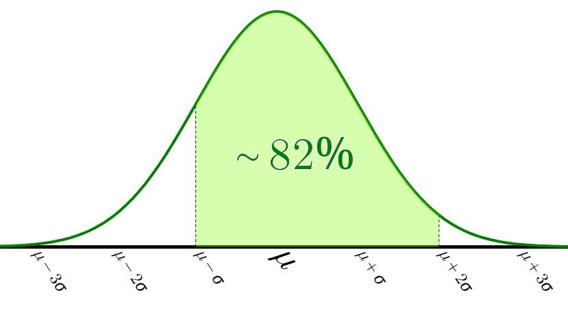
The standard normal distribution is often shifted and scaled
to have mean \(\mu\) and variance \(\sigma^2:\)
\[ \frac{1}{\sigma\sqrt{2\pi}}\mathrm{e}^{-\frac{1}{2}\bigl(\frac{x-\mu}{\sigma}\bigr)^2} \]
The expected value of \(X\), denoted \(\operatorname{E}\bigl(X\bigr)\)
and often simply referred to as the mean and denoted \(\mu,\)
is computed as \(\operatorname{E}\bigl(X\bigr) = \int_{D} x f(x) \,\mathrm{d}x\,.\)
The variance of \(X,\) denoted \(\operatorname{Var}(X)\) or \(\sigma^2,\)
is computed as \(\operatorname{Var}\bigl(X\bigr) = \int_{D} (x\!-\!\mu)^2 f(x) \,\mathrm{d}x\,.\)
The standard deviation of \(X\) is the positive square root of the variance,
and is denoted as \(\sigma.\)
The standard normal distribution is often shifted and scaled
to have mean \(\mu\) and variance \(\sigma^2:\)
\[ \frac{1}{\sigma\sqrt{2\pi}}\mathrm{e}^{-\frac{1}{2}\bigl(\frac{x-\mu}{\sigma}\bigr)^2} \]