Recall the distributive law in some of its forms: \( a(b+c)=ab+ac \) and \((a+b)(c+d)=ac+ad+bc+bd \) and \((a+b)^2 = a^2+2ab+b^2\,.\)
Recall the operation of exponentiation, where \(x^n\) denotes the product of \(x\) with itself \(n\) times, and recall these “rules” of exponentiation: \[ x^{0} = 1 \qquad x^a x^b = x^{a+b} \qquad (xy)^a = x^a y^a \qquad \bigl(x^a\bigr)^b = x^{ab} \qquad \biggl(\frac{x}{y}\biggr)^a = \frac{x^a}{y^a} \qquad x^{-a} = \frac{1}{x^a} \qquad x^{1/a} = \sqrt[a]{x} \qquad x^{a} = \frac{1}{x^{-a}} \qquad x^{a} = \sqrt[1/a]{x} \]
 After designating an origin point and two perpendicular coordinate axes
— conventionally an \(x\)-axis whose positive direction points eastward
and a \(y\)-axis whose positive direction points northward
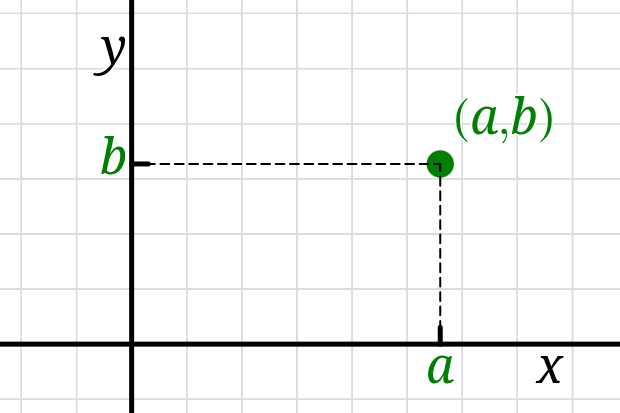
— we can describe the location of a point with its rectangular coordinates,
an ordered pair \((a,b)\) where \(a\) is its position in the \(x\) direction
and \(b\) is its position in the \(y\) direction.
Altogether this imbues the plane with a rectangular (Cartesian) coordinate system,
and we refer to it as the \(xy\)-plane.
After designating an origin point and two perpendicular coordinate axes
— conventionally an \(x\)-axis whose positive direction points eastward
and a \(y\)-axis whose positive direction points northward
— we can describe the location of a point with its rectangular coordinates,
an ordered pair \((a,b)\) where \(a\) is its position in the \(x\) direction
and \(b\) is its position in the \(y\) direction.
Altogether this imbues the plane with a rectangular (Cartesian) coordinate system,
and we refer to it as the \(xy\)-plane.
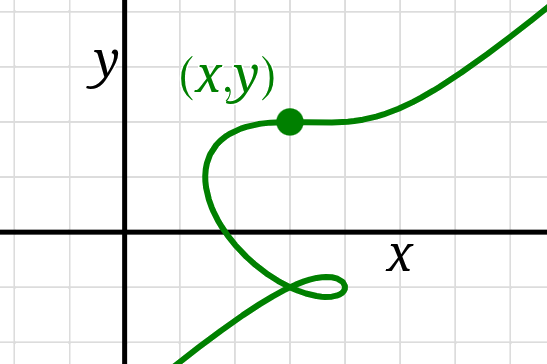 The solutions to any equation with two variables \(x\) and \(y,\)
the ordered pairs \((x,y)\) that make the equation true,
can be plotted in the \(xy\)-plane,
giving us a geometric perspective on the equation.
If the equation is “nice”, then that set of solutions will form
a connected curve in the \(xy\)-plane.
The solutions to any equation with two variables \(x\) and \(y,\)
the ordered pairs \((x,y)\) that make the equation true,
can be plotted in the \(xy\)-plane,
giving us a geometric perspective on the equation.
If the equation is “nice”, then that set of solutions will form
a connected curve in the \(xy\)-plane.