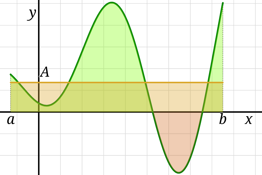
 The average value \(A\) of a function \(f\) on the interval \([a,b]\)
is computed by the formula
\[ A = \frac{1}{b-a}\int_a^b f(x) \,\mathrm{d}x\,. \]
This is the continuous analog of a typical discrete average:
“add up all the numbers and divide by how many numbers there were.”
The average value of the function \(f\) is also the unique number
that could replace \(f(x)\) as the integrand in the integral
without changing the value of the integral:
\(\int_a^b f(x) \,\mathrm{d}x = \int_a^b A \,\mathrm{d}x.\)
The average value \(A\) of a function \(f\) on the interval \([a,b]\)
is computed by the formula
\[ A = \frac{1}{b-a}\int_a^b f(x) \,\mathrm{d}x\,. \]
This is the continuous analog of a typical discrete average:
“add up all the numbers and divide by how many numbers there were.”
The average value of the function \(f\) is also the unique number
that could replace \(f(x)\) as the integrand in the integral
without changing the value of the integral:
\(\int_a^b f(x) \,\mathrm{d}x = \int_a^b A \,\mathrm{d}x.\)
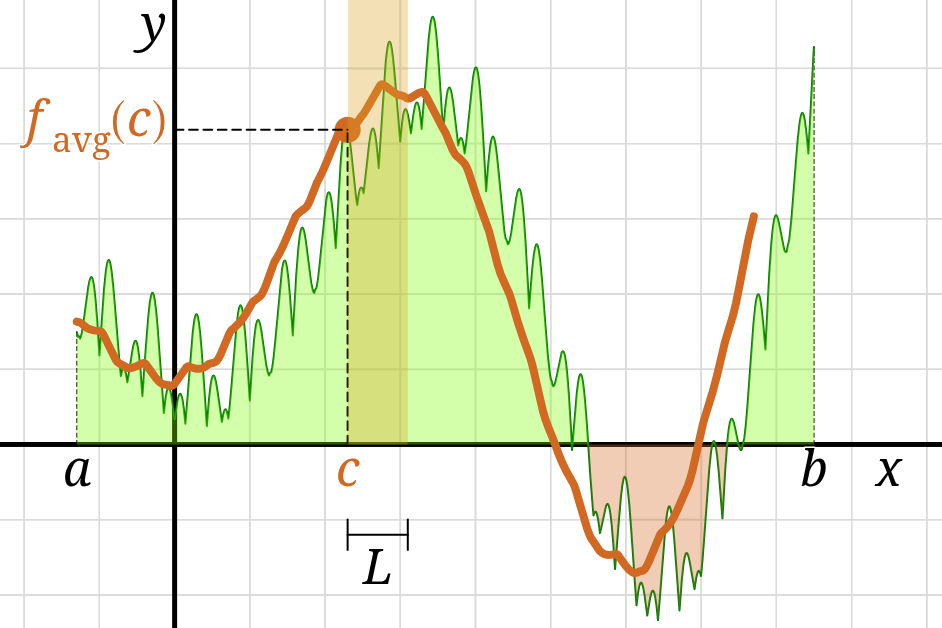 The moving average of a function \(f\),
also sometimes called a rolling average,
is a new function \(f_{\mathrm{avg}}\) defined by the formula
\[ f_{\mathrm{avg}}(x) = \frac{1}{L}\int\limits_{x}^{x+L}f(t)\,\mathrm{d}t \]
for some value of the parameter \(L\).
The output of \(f_{\mathrm{avg}}\) at every input \(x\) is the average value of \(f\)
on the interval of length \(L\) to the right of \(x.\)
The function \(f_{\mathrm{avg}}\) provides a smoother version of \(f,\)
which is helpful for analyzing “noisy” functions
that exhibit rapid fluctuation in the short-term
but appear to have a nice overall trend.
The moving average of a function \(f\),
also sometimes called a rolling average,
is a new function \(f_{\mathrm{avg}}\) defined by the formula
\[ f_{\mathrm{avg}}(x) = \frac{1}{L}\int\limits_{x}^{x+L}f(t)\,\mathrm{d}t \]
for some value of the parameter \(L\).
The output of \(f_{\mathrm{avg}}\) at every input \(x\) is the average value of \(f\)
on the interval of length \(L\) to the right of \(x.\)
The function \(f_{\mathrm{avg}}\) provides a smoother version of \(f,\)
which is helpful for analyzing “noisy” functions
that exhibit rapid fluctuation in the short-term
but appear to have a nice overall trend.